Convolution Neural Net practice with Keras (in tensorflow)

Convolutional Neural Nets (CNNs) are all the rage these days, being used anywhere from Health-related image analysis to Earthquake detection.
With all these amazing uses of this type of Neural Network, you may think that using CNNs for your own needs may be impossible...

With the help of Keras (and Tensorflow) it's actually fairly straightforward to begin developing a CNN.

What is convolution?

Previously, we worked with normal dense networks (where every node is connected). With convolution layers, we instead only connect our input nodes to some of the nodes in the next layer. This is easiest viewed as a matrix calculation, where we convolve our input nodes with our set of edges (we can call this set a filter) to produce a set of features.

We can view a set of edges as one filter. These edges will connect to the output feature map in different ways depending on how we setup the network. We accomplish this convolution by moving it across our input (typically an image).

The gif below (from This guide to CNNs) gives a good example of the convolution process. Here, we use a 3 X 3 filter with a stride of 1 (horizontal and vertical) on a 5 X 5 input matrix (or you could think about it at 25 nodes if flattened out) to create a 3 X 3 resulting matrix.

I'm going to walk through some code I wrote with the help of another Keras tutorial and the help of this tutorial for visualizing the filters on test data.

This should not be thought of as a state of the art, instead you should consider this a very gentle introduction without much partciular thought into particularly optimized or efficient , while also introducing you to one potential way to view a pitfall of not having heterogenous data.

Our libraries

With this example, we'll use keras and tensorflow libraries, as well as others to process & display images (cv2), process a csv file (csv), and display how our Neural Net did with a simple graph (matplotlib). We also use numpy so that we can manipulate matrices along the way (e.g., our images).

import tensorflow as tf
from tensorflow import keras
from tensorflow.keras.callbacks import TensorBoard, History
import numpy as np
import matplotlib.pyplot as plt
import math
import os
import os.path
import csv
import cv2
import random
import time

The FaceOff class

We create a class called FaceOff that processes images from the Chicago Face Database and tries to learn affective ratings based on training data. We use the name FaceOff to commemorate perhaps the greatest movie of all time, Face/Off

This is actually a pretty hilariously not great movie with all the expected 90s ridiculousness. I take no responsibility for wasted time

So for our FaceOff class, we'll start out with two simple class constants that will allows us to save our model along the way and a very simple constructor that we will use to hold our train & test data (images and corresponding affect ratings). This is important, because it allows us to not lose all the work of our Neural Net if we happen to have something crash at the end or we need to stop the model in the middle of it's training.

For more on saving your model (particularly in tensorflow), you can take look at this tutorial.

class FaceOff:

	CHKPT_PATH = "FO_training/cp-{epoch:04d}.ckpt"
	CHKPT_DIR = os.path.dirname(CHKPT_PATH)

	def __init__(self):
		self._test_images = []
		self._train_images = []

Getting our data

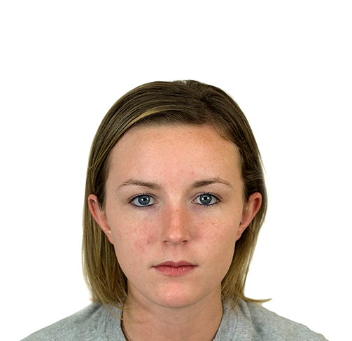
For this example, we will train on a subset of data and test our CNN on another subset.

Our dataset has images with have certain prefixes that allow us to know certain aspects of the image. The prefix (`target_prefix`) tells the race and sex of the participant in the image, while `target_fexpr`is used to only get certain expressions. In the case of `get_train_img_data`, we are getting images from White Females (WF) with a neutral (N) facial expression. The images (from the Chicago Faces homepage) below are an example of two images that you may see within the image set that fall under the Neutral category.

A white female with a neutral expression

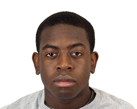
A black male with a neutral expression

If you happen to get the actual Norming Data, you'll notice that I read in a csv under a different assumed structure that the original data.
To simplify things, I've manually edited the norming data so that some of the original headers are gone and only column labels are present.


	#14 == angry row. 13-26
	def get_train_img_data(self, root_path, rating_filename = "CFD.csv", target_prefix="WF-", target_fexpr="-N"):
		'''
		Read train data (ratings + actual images) from specified directory
		'''
		img_rating_file = open(os.path.join(root_path, rating_filename))
		img_rr = csv.reader(img_rating_file)
		first_row = True
		img_ratings = dict()

		#Get our image ratings
		for row in img_rr:
			if (not(first_row)):
				#Only getting certain images for now
				if (row[0].find(target_prefix) != -1):
					#First column is our uid, use that as key to store rest of row
					# We are only worried about some of the affect ratings data
					img_ratings[row[0]] = row[12:26]
			else:
				first_row = False
				continue

		#now get our images
		img_dirs = [f for f in os.listdir(root_path)
					if os.path.isdir(os.path.join(root_path, f))
						and (str(f).find(target_prefix) != -1)]

		imgs = dict()

		for img_dir in img_dirs:
			img_files = [f for f in os.listdir(os.path.join(root_path,img_dir))
							if (os.path.isfile(os.path.join(root_path,img_dir,f))
								and (f.find(target_fexpr) != -1))]
			#We should only have one file/image (read that in using cv2)
			img_data = cv2.imread(os.path.join(root_path,img_dir,img_files[0]), cv2.IMREAD_COLOR)
			#(500,351) originally (2000, 1404)
			img_data = cv2.resize(img_data, (500,351))
			self._train_images.append([np.array(img_data), img_ratings[img_dir]])
		#Shuffle our training dataset
		random.shuffle(self._test_images)

The get_test_img_data method is very similar to the get_train_img_data. In fact, the only actual difference is that we're changing the defaults so that we actually get a different set of images


	def get_test_img_data(self, root_path, rating_filename = "CFD.csv", target_prefix="BM-", target_fexpr="-N"):
		'''
		Read test data (ratings + actual images) from specified directory
		'''
		img_rating_file = open(os.path.join(root_path, rating_filename))
		img_rr = csv.reader(img_rating_file)
		first_row = True
		img_ratings = dict()

		#Get our image ratings
		for row in img_rr:
			if (not(first_row)):
				#Only getting certain images for now
				if (row[0].find(target_prefix) != -1):
					#First column is our uid, use that as key to store rest of row
					# We are only worried about some of the affect ratings data
					img_ratings[row[0]] = row[12:26]
			else:
				first_row = False
				continue

		#now get our images
		img_dirs = [f for f in os.listdir(root_path)
					if os.path.isdir(os.path.join(root_path, f))
						and (str(f).find(target_prefix) != -1)]

		imgs = dict()

		for img_dir in img_dirs:
			img_files = [f for f in os.listdir(os.path.join(root_path,img_dir))
							if (os.path.isfile(os.path.join(root_path,img_dir,f))
								and (f.find(target_fexpr) != -1))]
			#print(img_files)
			#We should only have one file/image (read that in using cv2)
			img_data = cv2.imread(os.path.join(root_path,img_dir,img_files[0]), cv2.IMREAD_COLOR)
			img_data = cv2.resize(img_data, (500,351))
			self._test_images.append([np.array(img_data), img_ratings[img_dir]])

Creating the model

Now that we can load those data, let's move on to the difficult part: let's build our CNN. Below, we use keras located within the tensorflow framework. It should be noted that keras works on it's own and can be run with other frameworks (i.e., CNTK and Theano), so even if you don't want to specifically use tensorflow, this general tutorial will be useful (though the code itself may have slight differences).

In the code below, we first make it so our model will save it's place using the ModelCheckpoint method. We use the class constant mentioned previously to define where to save the model checkpoint, and we save the model every 5 (period=5) epochs.

self.cp_callback = tf.keras.callbacks.ModelCheckpoint(FaceOff.CHKPT_PATH, save_weights_only=True, verbose=1, period=5)

Now we can create our model. Below, I included two different ways that you can create your model.
Notice that we have a slightly different representation for input with the second version of the model. In the second version of the model formation, we create tensors and create a new model using those tensors as opposed to directly creating the model in the former (commented out) model development.

We increase the number of filters as we move along with our convolutions with the assumption that we get higher level features earlier in the process. Notice, we also have a kernal size of 3x3 kernel_size=3, a 2x2 stride strides=(2,2), and zero padding padding="same". We also have two dropouts in the model. As noted well in the Keras Documentation that also provides the actual academic reference for this mechanism, dropout will randomly set a fraction of previous layer units to 0.

input = keras.layers.Input(shape=(351,500,3))
self.model = keras.layers.Conv2D(filters=64, kernel_size=3, strides=(2,2),
	padding="same", activation="relu", name="conv1")(input)
self.model = keras.layers.MaxPooling2D(pool_size=(2,2), padding="same", name="mPool1")(self.model)
self.model = keras.layers.Conv2D(filters=128, kernel_size=3, strides=(2,2),
	padding="same", activation="relu", name="conv2")(self.model)
self.model = keras.layers.MaxPooling2D(pool_size=(2,2), padding="same", name="mPool2")(self.model)
self.model = keras.layers.Conv2D(filters=256, kernel_size=3, strides=(2,2),
	padding="same", activation="relu", name="conv3")(self.model)
self.model = keras.layers.MaxPooling2D(pool_size=(2,2), padding="same", name="mPool3")(self.model)
self.model = keras.layers.Dropout(0.25)(self.model)
self.model = keras.layers.Flatten()(self.model)
self.model = keras.layers.Dense(512, activation="sigmoid", name="dense1")(self.model)
self.model = keras.layers.Dropout(0.25)(self.model)
self.model = keras.layers.Dense(14, activation="relu", name="preds")(self.model)
self.model = keras.Model(inputs=input, outputs=self.model)

When we compile our model, self.model.compile(...), we have an opportunity to set an optimizer, a loss function, and what metrics we might want to use to measure how well our model is doing when we train it. This paper and corresponding blog post are great references for an optimizer; the visualization under the Visualization of algorithms heading towards the end of the blog post is useful. Mean squared error (mse) is used because we, essentially, have a regression problem (given the image we want to match the ratings as well as possible and be able to predict the same rating given an image with some unspecified features); if we were to be, say, classifying a dominant affect/emotion, then we would use a different loss function, perhaps categorical_crossentropy. We use AdaDelta because it gives us an adaptive learning rate, but only takes into account more recent results to adapt that learning rate (note that this allows us to contextualize within more recent results as opposed to keeping a completely global context to adapt our learning rate).

self.model.compile(optimizer="adadelta", loss="mse",
	metrics=["accuracy", "categorical_crossentropy"])

We also have an option to just set our model if we happened to load a model from a checkpoint


	def create_conv_model(self, model=None):
		'''
		Constructs a new model and assigns it or just assigns the model passed in.
		Also constructs
		'''
		self.cp_callback = tf.keras.callbacks.ModelCheckpoint(FaceOff.CHKPT_PATH, save_weights_only=True, verbose=1, period=5)
		if (model is None):
			'''self.model = keras.Sequential([
				keras.layers.InputLayer(input_shape=[351,500,3]),
				keras.layers.Conv2D(filters=64, kernel_size=3, strides=(2,2),
					padding="same", activation="relu", name="conv1"),
				keras.layers.MaxPooling2D(pool_size=(2,2), padding="same", name="mPool1"),
				keras.layers.Conv2D(filters=128, kernel_size=3, strides=(2,2),
					padding="same", activation="relu", name="conv2"),
				keras.layers.MaxPooling2D(pool_size=(2,2), padding="same", name="mPool2"),
				keras.layers.Conv2D(filters=256, kernel_size=3, strides=(2,2),
					padding="same", activation="relu", name="conv3"),
				keras.layers.MaxPooling2D(pool_size=(2,2), padding="same", name="mPool3"),
				keras.layers.Dropout(0.25),
				keras.layers.Flatten(),
				keras.layers.Dense(512, activation="sigmoid", name="dense1"),
				keras.layers.Dropout(0.25),
				keras.layers.Dense(14, activation="relu", name="preds")
			])'''
			input = keras.layers.Input(shape=(351,500,3))
			self.model = keras.layers.Conv2D(filters=64, kernel_size=3, strides=(2,2),
				padding="same", activation="relu", name="conv1")(input)
			self.model = keras.layers.MaxPooling2D(pool_size=(2,2), padding="same", name="mPool1")(self.model)
			self.model = keras.layers.Conv2D(filters=128, kernel_size=3, strides=(2,2),
				padding="same", activation="relu", name="conv2")(self.model)
			self.model = keras.layers.MaxPooling2D(pool_size=(2,2), padding="same", name="mPool2")(self.model)
			self.model = keras.layers.Conv2D(filters=256, kernel_size=3, strides=(2,2),
				padding="same", activation="relu", name="conv3")(self.model)
			self.model = keras.layers.MaxPooling2D(pool_size=(2,2), padding="same", name="mPool3")(self.model)
			self.model = keras.layers.Dropout(0.25)(self.model)
			self.model = keras.layers.Flatten()(self.model)
			self.model = keras.layers.Dense(512, activation="sigmoid", name="dense1")(self.model)
			self.model = keras.layers.Dropout(0.25)(self.model)
			self.model = keras.layers.Dense(14, activation="relu", name="preds")(self.model)
			self.model = keras.Model(inputs=input, outputs=self.model)


			self.model.compile(optimizer="adadelta", loss="mse",
				metrics=["accuracy", "categorical_crossentropy"])
		else:
			self.model = model

Here we are just loading an assumed saved model using model_weights; this means that we have to have already created a model instance with the same structure as our weights!


	def load_model(self, model_weights):
		self.model.load_weights(model_weights)

Training the model

As we have the ability to create our model, perhaps we should create the functionality to train it!

The first thing we do below is get our images and corresponding ratings out separately so that we can use the images as inputs x_imgs and the affective ratings as outputs x_ratings. We will use both the test_ and train_ objects in the model fitting.

Next, we create our history object that will be used to save our history along the way and allow us to plot the history afterwards. The model.fit is where our action is as far as training our model goes. We set our input, x to be the training images tr_imgs and our output, y, to be the corresponding ratings tr_ratings. We also specify a batch size (see this previous link for more on types of gradient descent, including mini-batch descent.) Lastly, we provide the history object as a callback so that the system knows to keep track of the learning history using that object and we supply validation_data so that we can keep track of how well our model is performing with those data we might use to validate (or in this case test) the model once it's trained.

Afetr the model is trained, we give a summary of the training with model.summary(). Finally, we plot the history of the training itself using our plot_history function.

	def train_model(self):
		tr_imgs = np.array([x[0] for x in self._train_images])
		tr_ratings = np.array([x[1] for x in self._train_images])

		tst_imgs = np.array([x[0] for x in self._test_images])
		tst_ratings = np.array([x[1] for x in self._test_images])

		history = History()
		self.model.fit(x=tr_imgs, y=tr_ratings, batch_size=50, epochs=1000, callbacks=[history, self.cp_callback],
			validation_data=(tst_imgs, tst_ratings))
		self.model.summary()
		self.plot_history([("ConvNet", history)])

	def plot_history(self, histories, key="acc"):
		plt.figure(figsize=(16,10))

		for (name, history) in histories:
			val = plt.plot(history.epoch, history.history["" + key],
				"--", label=name.title() + " Val")
			#print(history.history["" + key])
			plt.plot(history.epoch, history.history[key], color=val[0].get_color(),
				label=name.title() + " Train")

		plt.xlabel("Epochs")
		plt.ylabel(key.replace("_", " ").title())
		plt.legend()
		plt.xlim([0,max(history.epoch)])
		plt.show()

Some methods to help us understand

If we happen to want to understand the process of a convolution layer a bit more and practice by writing things out by hand, we can use the function below. This uses the values for input and filter matrices that I went over in class and prints out the resulting weights. Notice that we use mean absolute error as our loss function so that we can get the same numbers we used in class. Also notice the `kernal_size` and `strides` parameters, which create a 2X2 filter that moves horizontally and vertically one row & column a time.


	@staticmethod
	def understand_conv_process():
		'''
		Apparently tensorboard exists, and will probably be more useful...but sunken cost and all
		'''
		model = keras.Sequential([
			keras.layers.Conv2D(filters=1, kernel_size=(2,2), strides=(1,1),
				padding="valid", input_shape=(3,3,1))
			#keras.layers.MaxPooling2D(p)
		])
		#Manually set our weights so that we can test!
		w_arr = [np.array([[[[0.5]],[[0.6]]],[[[0.7]],[[0.8]]]]),np.array([0.])]
		model.set_weights(w_arr)
		print(model.get_weights())
		model.compile(optimizer=keras.optimizers.SGD(lr=.2), loss="mae", metrics=["accuracy"])

		x = np.array([[1, 1.1, 1.2],[0.9, 0.8, 0.7],[0.5, 0.6, 0.4]])
		x = np.expand_dims(x, axis=2)
		x = x.reshape((1,3,3,1))
		yd = np.array([[1,3],[2,4]])
		yd = np.expand_dims(yd,axis=2)
		yd = yd.reshape((1,2,2,1))
		history = History()
		model.fit(x,yd, batch_size=1, epochs=1, verbose=1, callbacks=[history])
		print(history.history)
		print(model.get_weights()[0])
		print(model.total_loss)

We can also use the functions below to show how that particular layer might see an image after trained. The plot_filter method can be used to look at layers independently, or the plot_filters method might be used as a shortcut to plot several convolution layers. To have more details see This helpful tutorial which is what the code is based on.


	#Static method to display what a layer is outputting based on test image
	# Used https://www.codeastar.com/visualize-convolutional-neural-network/ with own modifications
	@staticmethod
	def plot_filter(model, nrows, ncols, layer, tst_img):
		#Create a model with all layers up to particular convolution layer
		a_model = keras.Model(inputs=model.input, outputs=model.get_layer(layer).output)
		a_model_out = a_model.predict(np.expand_dims(tst_img, axis=0))
		(fig, ax) = plt.subplots(nrows, ncols, figsize=(nrows*2.5, ncols*1.5))
		filt_ind = 0
		loop_err = False
		#Show our test image passed through all of the filters in this convolution layer
		for i in range(nrows):
			for j in range(ncols):
					ax[i][j].imshow(a_model_out[0,:,:,filt_ind], cmap="gray")
					filt_ind += 1
		plt.show()

	def plot_filters(model, nrows, ncols, tst_img):
		for layer in model.layers:
			if ("conv" in layer.name):
				num_filters = layer.output_shape[3]

				#Find a reasonable number of rows & cols for plot
				nrows = math.ceil(math.sqrt(num_filters))
				if (num_filters % nrows != 0):
					while (num_filters % nrows != 0):
						nrows -= 1
				ncols = int(num_filters/nrows)

				#plot the current convolutional layer
				FaceOff.plot_filter(model, nrows, ncols, layer.name, tst_img)

Below is just some code to use our methods (get those data, construct the model, train the model, plot the model filters)
This code also includes commented out lines that would allow us to load the last saved model for use, which we would swap with test_conv.train_model() if we had already trained a model that we would like to use.


keras.backend.set_session(tf.Session(config=tf.ConfigProto(intra_op_parallelism_threads = 28, inter_op_parallelism_threads = 28)))
test_conv = FaceOff()
test_conv.get_train_img_data("../../TF_Test/CFD/")
test_conv.get_test_img_data("../../TF_Test/CFD/")
test_conv.create_conv_model()
#last_model = tf.train.latest_checkpoint(FaceOff.CHKPT_DIR)
#test_conv.load_model(last_model)
tst_imgs = np.array([x[0] for x in test_conv._test_images])
test_conv.train_model()
FaceOff.plot_filters(test_conv.model, 3, 5, tst_imgs[0])

There's plenty more you can do (and tons of tutorials & references out there besides the ones that I posted), but hopefully this was a nice gentle introduction to something that can on the surface seem daunting and now you fill the pull of working with some of these AI algorithms on your own!

Ok....maybe I wrote that last sentence just so that I could end with this GIF...