The assignment was for the creation of the entire automated proceedure
from two images to the Fundamental Matrix F, using a corner detector,
correspondence selector (ZNCC, SSD), RANSAC with 7-point and
8-point solvers, non-linear optimization on linear results, and
guided
matching using the best computed F's.
This was a lot of code.
corner_detector.m
find_correspondences_ZNCC.m
drawCorrespondences_ZNCC.m
find_correspondences_SSD.m
computeF_8point.m
computeF_RANSAC.m
computeF_7point_ransac.m
drawInliers.m
reestimateF.m
basic_cost_nonlin.m
sampson_cost_nonlin.m
guided_matching_ZNCC.m
selectEpipolarLines.m
compute_residual.m
ComputeF_All.m
I'll go through an example, then conclude.
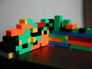
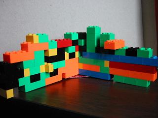
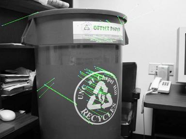
First I looked at a slightly translated and rotated
pair of images, of a lego wall.
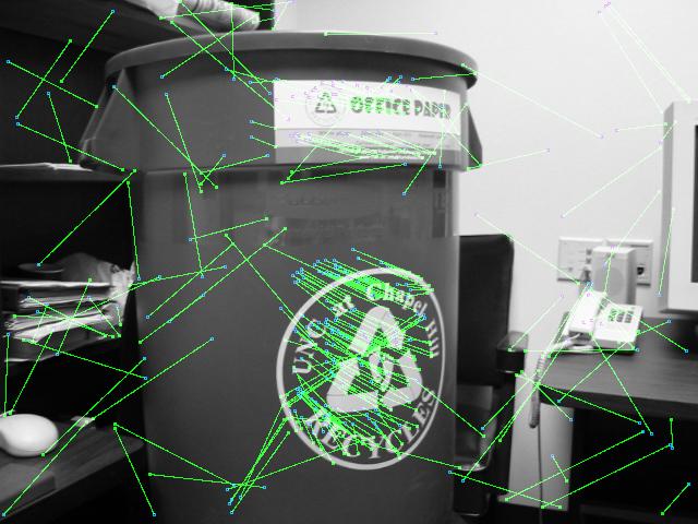
The feature point selection found approximately 800 points of interest.
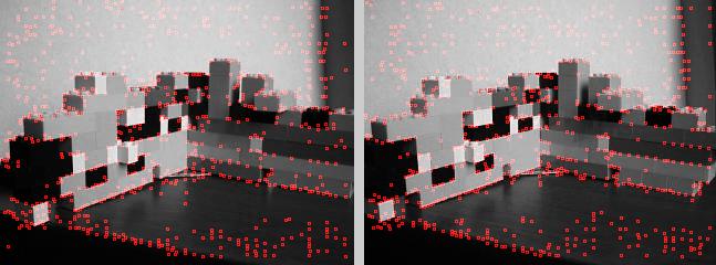
Upon Zero-Mean Normalized Cross-Correlation, using
a large (31x31) patch size and high
threshold for reasonable correspondences (.7), there were 327 correspondences.
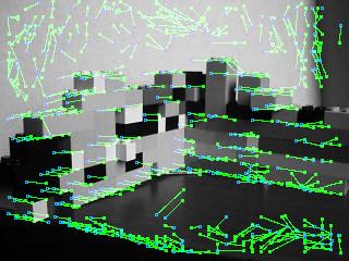
On the left is result of the ZNCC algorithm.
As can be observed, there are still outliers,
but in all good correspondences. On the right is the results
from a SSD computation. I
could not find a way to discriminate between bad and good among
the good matches using
SSD. In ZNCC, the minimum response made sense as a way to
determine if a match was
really good or just happenstance. However, with SSD, even
after equalizing the intensity
profiles of the two images, a comparable maximum allowable response
did not improve
the results. In that ZNCC works well though, I did not search
very hard.
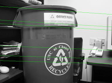
Here is the result (on the left) of the normalized
8 point algorithm, and (on the right) the
solution with a random 7 points among them using the minimum solution. 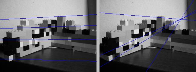
Obviously, a random seven correspondences does
not give an ideal solution.
The residual, or the average symmetric epipolar
distance, on the 8 point algorithm over
all the correspondences was 22.0044. For the random solution,
114.4158.
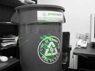
Next, we perform the RANSAC algorithm, the point
of which is to pick a random seven
correspondences whose seven-point solution contains the largest
number of inliers one
could expect. RANSAC discovered a seven point solution for
which 211 of the 327 (66%)
correspondences were inliers (within one pixel).
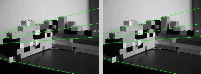
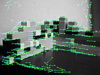
The two images show epipolar lines computing
using the best case F from the RANSAC
algorithm, and the 8 point normalized solution using the correspondences
determined by
RANSAC to be inliers. They are virtually identical, as might
be expected. The residual for
the F returned from RANSAC is .5395, while the 8 point algorithm
computes an F with
residual .4675. These residuals were for correspondences that
were determined inliers.
From now, we use only the inliers to better our
results. In non-linear optimization, a rule
of thumb is to initialize the non-linear step with something pretty
much the solution (which
is funny). In my optimizations, the points were fixed.
I used lsqnonlin with two different cost functions.
The first function computes the two
terms in the symmetric epipolar distance and averages them (their
square roots actually,
so just epipolar distances), for each point. The cost functional
returned to lsqnonlin is then
a column vector of average error for each correspondence.
The second cost function was the Sampson error
computed as (xp'*F*x)^2 divided by the
four part sum of the square magnitudes of F*x and F'*xp. This
again was computed for
every correspondence and returned as a column vector. Since
lsqnonlin squares the results
again, these numbers may have been quite small, leading to the optimization
stopping short.
The two F matrices computed in this way differred
very slightly from the 8 point solution
(above) that they were initialized to. For the Sampson error
cost function, the residual on
the inliers was .4670, while the residual using my distance metric
was .4618, both slightly
better than the residual in their initialization.
The book notes that the Sampson error is first
order approximation to geometric error.
My cost function is actual perpendicular point to epipolar line
distance, and so might be
expected to give similar results.
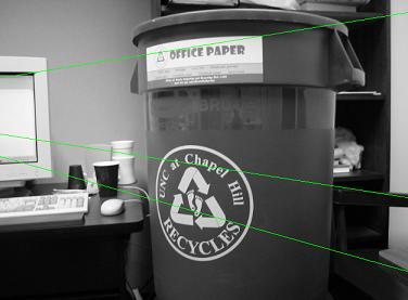
Next, I take the resultant F to compute epipolar-limited
point correspondences using
guided matching, on the original feature lists, to come up with
more correspondences that
would be inliers for that F.
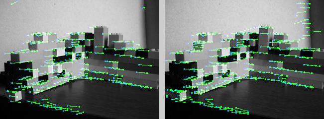
On the left is a picture of the inliers determined
by the RANSAC algorithm (for the best F).
On the right are all the correspondences determined by guided matching
using the F from the
non-linear optimization. There were 211 inliers for RANSAC,
and for the optimized F 260
good correspondences were found. It is clear that there may
still be some mismatches, but
now very few. Potential matches must be within one pixel of
the relevant epipolar line. After
non-linear restimation with these guided matches, a solution matrix
was obtained with a
residual of .4500. The residual is obviously dependent on
how close the potential matches
must be in the guided matching stage. There is probably something
in Nyquist theory that
can show that better-than .5 pixel residual is abberation, so I
didn't try to continue.
This was an interesting assignment. There
is a lot to it, but it seems like it ends without
much accomplished. I look forward to using the methods I have
now written to compute the
real 3D geometry.
Below is another example, this pair of images more disparate than previously.

The 8 point normalized has a residual of about 3000 (whew!).
After RANSAC, the best seven point solution has residual 1.17, and
the 8 point normalized has
residual only 1.01 (where inlier are within 2 pixels).
After non-lin optimization, the residue doesn't improve, going to
1.13.
The guided correspondence gives fewer correspondences than were
in the inliers set.
The computed epipolar geometry does look good in the area where the
inliers are, as would
be expected, and gets pretty bad farther away.
-Stough