Final Project: Jittered Supersampling with Area Light
Sources And
An Implementation of Mitchell's SIGGRAPH '87 Paper
All the matlab files:
raytrace_with_planes2.m
mitchell_raytrace.m
single_raytrace.m
g2d.m
Pwfi.m
intersect.m
p_intersect.m
Introduction:
For my final project, I wanted to make better looking
images come out of my very limited raytracer.
Specifically,
I looked to dampen aliasing effects caused by discrete sampling and
hard shadows caused by point light sources.
There are two approaches that I have implemented, a jittered supersampling
approach and a contrast-driven super-
sampling approach that is more effiecient for similar output.
I will discuss these in order.
Jittered Supersampling with Area Light Sources
The raytrace_with_planes2.m matlab file allows the
user to specify the object space, resolution, supersampling
resolution, and the support of gaussian blur used in the reconstruction.
Here is how the method works:
-Create an image of resolution*n^2
jittered samples, where n is the resolution multiplier the user specified.
The n^2 samples per pixel
are from randomly generated (uniform distrobution) rays in the pixel area.
Further,
the shadow rays cast upon
intersection are jittered in their direction, to approximate an area light
source. The
multiple samples per pixel
allows a nice averaging to take place in the penumbra (area barely in shadow).
-Reconstruct the final image
from the samples. The user-specified support for the gaussian filter
is in terms of
the final image pixels.
The filter is applied over 3x3 pixel areas to obtain the final image.
The issues I ran in to were in reconstruction. The gaussian serves
as a weighted average filter around a pixel. But
in order to know how to weight a particular sample in the support area,
we needed to remember where that
sample's ray jittered to, as it was randomly placed within the pixel's
area. Also, the sum of all the weights used in
the calculation of a pixel value must be 1 in order to avoid flooding
or dimming, no matter how many samples
were involved in the calculation (as there are fewer along the edges
of the image). Lastly, I noticed that gaussian
used in reconstruction, if too large, produces badly blurred pictures,
while if too small, leaves aliasing in the image.
It was difficult to find a balance.
The program creates good looking images. I
noticed a tradeoff in the number of samples per pixel verses the
extent of penumbras in the image. A large area light source produces
speckle in the penumbra unless (I believe)
exponentially more samples are cast per pixel. Also, though the
distrobution over the pixel's area is supposed to
be uniform, I found that a jaggy effect still occurs in the jittered
supersampled image (see figure 3). I cannot
explain this except to say that tying what should be a random ray's
direction to the center of a pixel may lead to
non-uniformity in the overall image's sample distrobution. Below
are example outputs.

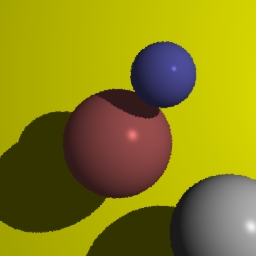
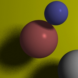
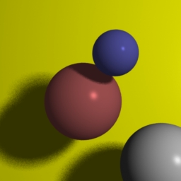
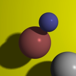
Figure1: (left to right, top to bottom) Progression of scene.
1. Classic one sample per pixel ray trace. 2. Filtered
with a gaussian in an attempt to ease the hard shadows.
3. 64 jittered samples per pixel with a large
area light source. 4 and 5. Successively smaller light sources
to lessen the speckle found in 3. Image 5 looks great.
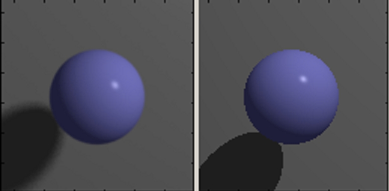
Figure 2: Closeup for comparison. On the left is my program,
on the right the original raytracer.
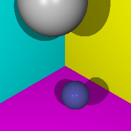

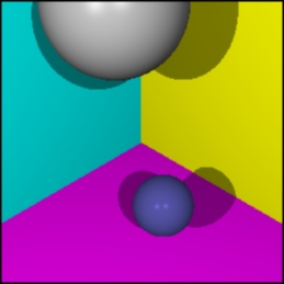
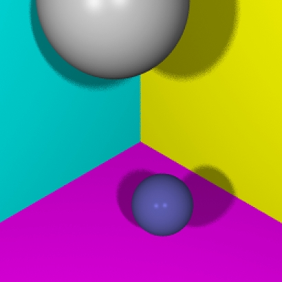
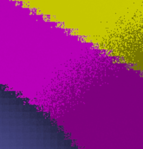
Figure 3: 1. Original raytracer output. 2. My program's
better output. 3. Original convolved with a small filter.
4 and 5. A very small version of the
jittered supersample image and a closeup.
The jittering was at 64 samples per pixel, and the output is a 256x256
image, so 4 is a 12 MB bitmap.
Notice a jaggy effect is visible, though noisier
than it would be otherwise. In that I could spread around the dots
on one of these borders in a way
that would make a nicer image, I feel this supersampled
jittering may not produce an ideal distrobution (lead in to Mitchell's
stuff below). However,
it may just be a programming artifact (I explain):
this jitter image is stored as a 2d array and while the rays cast being
stored in the array are grouped
by the pixel they belong to, there is no garanteed
order within the samples for a pixel--they are just random jitterings from
the center of the pixel.
This sounds convincing.
An Implementation of Don Mitchell's SIGGRAPH '87 Paper
("Generating Antialiased Images at Low Sampling Densities")
This was a cool paper and easy to understand.
One of the few papers where implementation details were not
completely dense (kinda makes you wonder why it would be accepted).
There are three parts to the implement-
ation, which I will go over in order: low density initial sampling,
contrast-driven local supersampling, and reconstr-
uction. We start with by setting a grid over the image we are
making that is "4 times finer than the display pixel
lattice (i.e., there are 16 grid points per pixel area)" (p.66).
We will work with this sampling space throughout.
As we made note of above, uniform distrobution jittered
sampling may not be ideal, and much work has been
put into finding a good all-purpose sampling. Mitchell uses efficiently
generated Poisson-disk samples as a low
density initial sampling of the object space, averaging about 1 sample
(out of the 16 possible) per pixel. The
equations quickly are (for a potential sample point):
T
= (4*D(i-1,j) + D(i-1,j-1) + 2*D(i,j-1) + D(i+1,j-1))/8 + (random in range
(1/16 +- 1/64))
SELECT = {0(no) is T < .5; 1(yes) otherwise}
D(i,j) = T - SELECT
 the
X's are determining factors in whether or not O will be an initial sample.
the
X's are determining factors in whether or not O will be an initial sample.
So what are related to diffusion values for previous potential samples
are combined to determine a diffusion for
the current potential sample and decide whether to take a sample at
the current place. The resultant sparse (in
terms of the 16 grid points per pixel lattice) sampling can now be
tested for high-contrast areas.
We would like to supersample in areas of high contrast
in order to keep as accurate information as possible
about the space we're imaging. For the samples within a 3x3 pixel
area (or 12x12 in the finer lattice), find the
following contrast for the three color channels:
C = (Imax-Imin) / (Imax+Imin)
The thresholds for each channel have been found experiementally: .35,
.25, .5 for red, green, blue respectively.
If the threshold is passed for a particular area, then randomly choose
another 8 or 9 samples per pixel in the
area (so 72 more than are already the low density samples we just considered).
There are two potential problems with my implementation
here. First, the contrast testing window is not
moving smoothly throughout the samples--the windows are non-overlapping
(as can be seen by the square
supersampling areas below). This may introduce (or keep) some
of the same aliasing problems we are trying to
get rid of. However, this would only leave blurred splotchiness
as evidence, where areas that maybe should
have been supersampled were just barely missed (notice that there is
not a continuous supersampling of the
planar intersections in figure 5 below). Secondly, I pick the
72 more samples in an area I wish to supersample
by uniformly distributed randomness, selecting a grid point for sampling
if I have not picked it yet. This may
introduce into the supersampling the same element of uniform distrobution
that above created the noticeable
jaggies in the jittered sampling. The images look good however,
and I am not sure how this potential problem
would express itself in the end.
The final stage is reconstruction. This is
done with the application of successively larger weighted-average
filters, because of the properties Mitchell found them to have in terms
of alliasing, as well as so that dense
sampling does not dominate final color computation. First we
apply a half-pixel squared (or 4 fine grid points)
filter on the samples. We don't include unsampled grid points
in the computation (they are not considered
zero). This leaves an image of point samples that have spead
out a little. Apply the filter again and the samples
get even wider support. The last step is a full pixel averaging--so
over the 16 grid points and their samples (if
they were sampled) per pixel, simply average. One may wonder
why the support of this last averaging filter is
only one pixel and not more as would usually be required to produce
antialiased images. The successive app-
lications of the 2x2 filter took care of introducing color elements
from neighboring pixels.
There were only a couple of issues I ran into in
implementing this part. First, as with the gaussian reconst-
ruction in the previous section, we need to remember how many and which
samples were in a given filter app-
lication, so that we can normalize the sum of weights to prevent flooding
or dimming. Secondly, the 2x2 filter
I apply twice computes under this support:  ,
where XO is the sample value being recomputed, based
,
where XO is the sample value being recomputed, based
on all four. In that I always apply this filter left to right,
top to bottom, I may be accentuating (or dampening
less) certain image attributes (the weights clockwise from XO might
be .4 .22 .22 .16 for example). It might
be cool to apply the filter once left-right-top-bottom, and then the
second application be right-left-bottom-top.
This may make the support of the overall filtering a little wider for
better smoothness (though more blur). In
fact, this dilemma is similar to the Poisson-disk sample generating
done above, where Mitchell mentions that
scanning back and forth (like an ox on a field...) instead of left
to right all the time may help isotropy (though
he did not implement it). Also, the filters applied during the
reconstruction are smoothly convolved with the
samples (the windows do overlap, not as before for the supersampling).
Lastly, I just want to note that after
spending hours making small changes to the coefficients in the averaging
filters, I gained almost no additional
intuition about the reconstruction phase (all the pictures look pretty
similar, regardless of variation in the
weights).
And that is my implementation of Mitchell's
low sample density antialiased image creation algorithm.
Example figures are shown below.
Conclusion
For my final project, I looked into ways I could
make my simple raytracer produce prettier pictures, in terms
of aliasing and hard shadows. Firstly, I implemented a (user
specified) high density jittered supersampling
approach with jittered light vectors to simulate area light sources.
I got good results but was dissappointed by
the excessive computation and the easy-to-overblur nature of the algorithm.
In response I implemented an algorithm described
by Mitchell in a SIGGRAPH '87 paper. I end up with
similar quality pictures at a small fraction of the computational cost
of my first program. There is very little
aliasing and much less blur than before. But I have come to believe
that we can never really finish the job of
making the best image possible, as there are so many directions to
look for it in, with different sampling and
supersampling and reconstruction techniques.
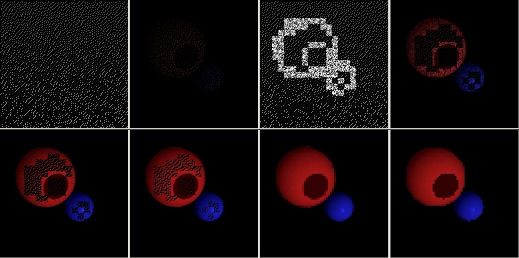
Figure 4: Progression of Mitchell's algorithm: A grid at 4x final resolution
will be non-uniformly sampled. 1. Low density Poisson disk sampling
points (~1.2 samples per pix).
2. The low density initial sampling (look closely).
3 and 4. Contrast driven adaptive supersampling (~8 additional samples
per pixel) and the resultant samples. 5 and 6.
Successive applications of a two by two (half pixel
squared, in terms of the final resolution) weighted-average filter.
7. Application of the 4x4 (full pixel) box filter. 8. The
classic raytraced image, for comparison. 7
and 8 are 64x64 pixel images shown at the supersampling resolution of the
others.
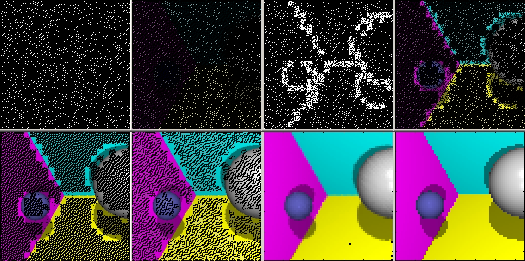
Figure 5: Same progression of Mitchell's algorithm as above.
I believe the empty dots in the seventh image (the final image in the progression)
are because of areas that were
completely empty of samples, which is pretty unlikely.
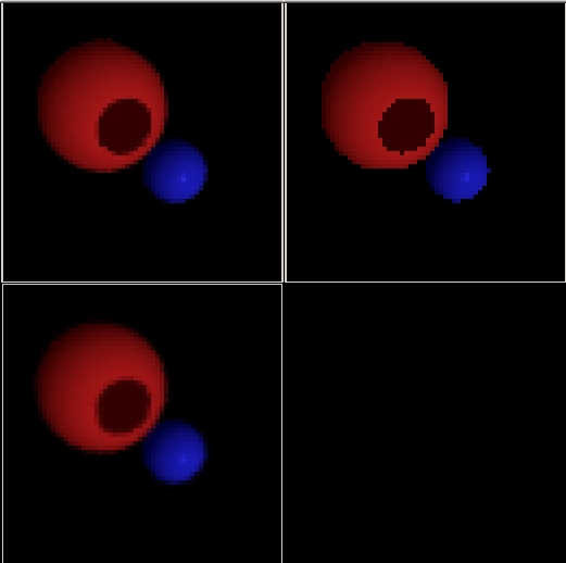
Figure 6: (clockwise) comparison of Mitchell's, classic single sample
per pixel, and my
16 sample per pixel (no matter what) approach from
above. Of course, my Mitchell
implementation provides similar quality for a small
fraction of the raytracing time.
Think of the last approach as having a pure-white
sampling density in the figure 4
progression above.
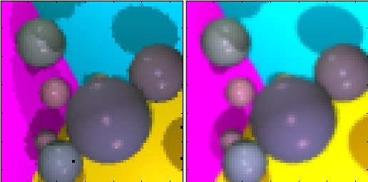
Figure 7: My Mitchell implementation (left) verses my raytrace_with_planes2.m.
The
images are at 64 pixel resolution, zoomed in for
better comparison. I would say
that they are similar enough for the fraction of
computation that Mitchell's requires.